Read Multiple Csv Files for Knn Classification
MultiClass Nomenclature Using K-Nearest Neighbours
In this article, learn what is multi-grade nomenclature and how does is work
![]()
INTRODUCTION:
Nomenclature is a classic machine learning awarding. Nomenclature basically categorises your output in 2 classes i.e. your output can be ane of two things. For example, a bank wants to know whether a client volition exist able pay his/her monthly investments or not? Nosotros tin can use machine learning algorithms to determine the output of this problem, which volition be either Yep or No(Ii classes). But what if you want to classify something that has more than 2 categories and isn't as unproblematic as a yes/no trouble?
This is where multi-course classification comes in. MultiClass classification can be defined as the classifying instances into one of iii or more classes. In this article we are going to do multi-class classification using Yard Nearest Neighbours. KNN is a super simple algorithm, which assumes that like things are in close proximity of each other. So if a datapoint is near to another datapoint, it assumes that they both belong to similar classes. To know more than deeply near KNN algorithms, I would suggest yous go check out this article:
Now, that we are through all the basics, permit's get to some implementation. We are going to utilize multiple python libraries like pandas(To read our dataset), Sklearn(To train our dataset and implement our model) and libraries like Seaborn and Matplotlib(To visualise our data). If you don't already accept this libraries install y'all tin can install them using pip or Anaconda on your pc/laptop. Or another way that I would personally suggest, utilize google colab to perform the experiment online with all the libraries pre-installed. The dataset that we are going to be using is called the IRIS blossom dataset and it basically has 4 features for it's 150 data points and is categorised into 3 unlike species i.due east. 50 flowers of each species.The dataset can be downloaded from the following link:
At present as we get started with our code, the outset step to practise is to import all the libraries in our code.
from sklearn import preprocessing from sklearn.model_selection import train_test_split from sklearn.neighbors import KNeighborsClassifier import matplotlib.pyplot as plt import seaborn as sns import pandas every bit pd
Once you've imported the libraries the next step is to read the information.Nosotros will use the pandas library for this function. While reading, nosotros will also check if there are any null values as well every bit the number of dissimilar species in the data. (Should be 3 equally our dataset has 3 species). Nosotros volition as well assign all the iii species categories a particular number, 0,i and 2.
          df = pd.read_csv('IRIS.csv')
df.caput() 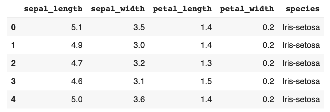
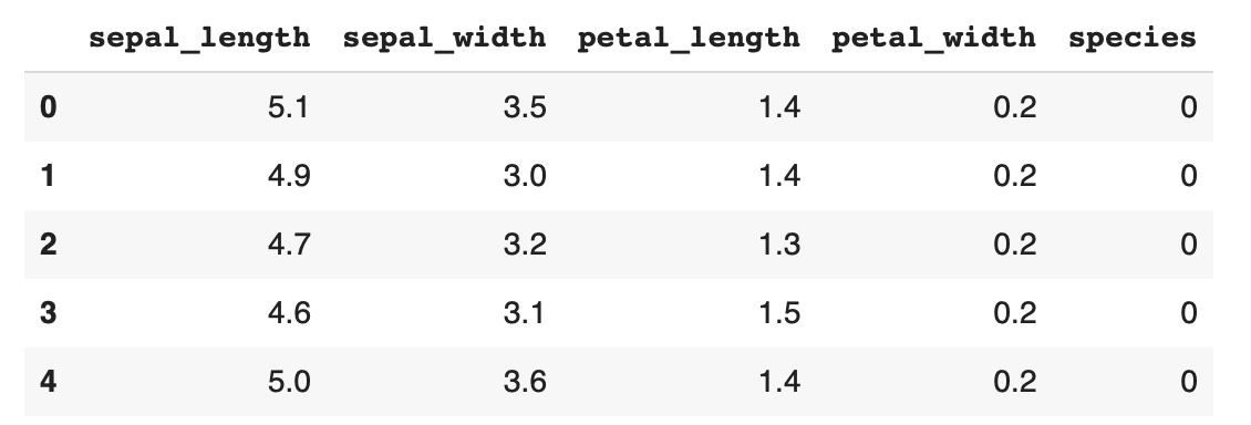
df['species'].unique() Output: array(['Iris-setosa', 'Iris-versicolor', 'Iris-virginica'], dtype=object)
df.isnull().values.whatsoever() Output: False
df['species'] = df['species'].map({'Iris-setosa' :0, 'Iris-versicolor' :one, 'Iris-virginica' :two}).astype(int) #mapping numbers df.head()
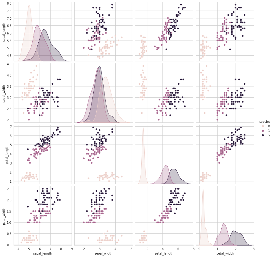
Once, that we are at present done with importing libraries and our CSV file, the side by side step we do is exploratory data analysis(EDA). EDA is necessary for any problem as it helps u.s.a. visualise the information and infer some conclusions initially simply by looking at the information and not performing whatever algorithms. We perform correlations between all the features using the library seaborn besides equally plot a scatterplot of all the datasets using the same library.
plt.close(); sns.set_style("whitegrid"); sns.pairplot(df, hue="species", height=3); plt.show()
Output:
sns.set_style("whitegrid"); sns.FacetGrid(df, hue='species', size=five) \ .map(plt.scatter, "sepal_length", "sepal_width") \ .add_legend(); plt.bear witness()
Output:

Inferences from EDA:
- While Setosa can be hands identified, Virnica and Versicolor have some overlap .
- Length and Width are the well-nigh important features to identify diverse flower types.
Later on the EDA and before training our model on the dataset, the ane last thing left to exercise is normalisation. Normalisation is basically bringing all the values of different features on a aforementioned calibration. As different features has different scale, normalising helps usa and the model to optimise it's parameters more efficiently. We normalise all our input from scale: 0 to 1. Hither, Ten is our inputs(hence dropping the classified species) and Y is our output(3 classes).
x_data = df.drop(['species'],axis=i) y_data = df['species'] MinMaxScaler = preprocessing.MinMaxScaler() X_data_minmax = MinMaxScaler.fit_transform(x_data) information = pd.DataFrame(X_data_minmax,columns=['sepal_length', 'sepal_width', 'petal_length', 'petal_width']) df.caput()

Finally, we have reached to the point of training the dataset. We use the built-in KNN algorithm from sci-kit acquire. Nosotros split the our input and output data into grooming and testing data, every bit to train the model on grooming data and testing model'southward accuracy on the testing model. We choose a 80%–20% divide for our training and testing data.
X_train, X_test, y_train, y_test = train_test_split(data, y_data,test_size=0.2, random_state = 1) knn_clf=KNeighborsClassifier() knn_clf.fit(X_train,y_train) ypred=knn_clf.predict(X_test) #These are the predicted output values
Output:
KNeighborsClassifier(algorithm='car', leaf_size=xxx, metric='minkowski', metric_params=None, n_jobs=None, n_neighbors=v, p=2, weights='uniform')
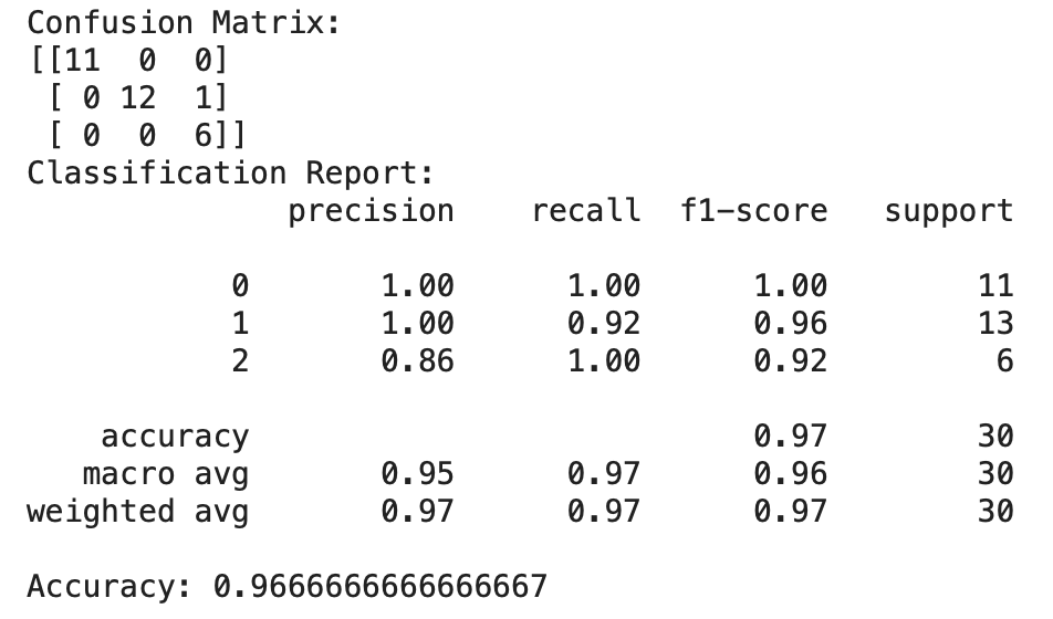
Here, we see that the classifier chose 5 as the optimum number of nearest neighbours to classify the information best. At present that we take built the model, our concluding stride is to visualise the results. We summate the confusion matrix, the precision recall parameters and the overall accuracy of the model.
from sklearn.metrics import classification_report, confusion_matrix, accuracy_score outcome = confusion_matrix(y_test, ypred) print("Defoliation Matrix:") print(result) result1 = classification_report(y_test, ypred) impress("Classification Report:",) print (result1) result2 = accuracy_score(y_test,ypred) print("Accurateness:",result2)
Output:
Summary/Conclusion:
Nosotros successfully implemented a KNN algorithm for the IRIS datset. We establish out the most impactful deatures through out EDA and normalised our dataset for improved accurateness. We got an accuracy of 96.67% with our algorithm every bit well as we got the defoliation matrix and the classification written report. From the classification report and the confusion matrix we tin can see that it misidentifies versicolor equally virginica.
That is how one tin do multi-course classification using KNN algorithm. Hope you learned something new and meaningful today.
Thank you.
sorensonwhoube1981.blogspot.com
Source: https://towardsdatascience.com/multiclass-classification-using-k-nearest-neighbours-ca5281a9ef76