Draw Null Clines in the Xy Phase Plane
phaseR: An R parcel for stage airplane analysis of one and two-dimensional autonomous ODE systems [one]. The phaseR bundle uses stability analysis to classify equilibrium points.
Fixed Points and Phase Portraits
Equilibrium points and stability. Equilibrium points of an autonomous ODE are defined at \(ten^*=0\) such that \(f(x^*)=0\). Why practise nosotros want to find the equilibrium points? Outset at a point \(x^*\) such that \(f(x^*)=0\), the arrangement, if unperturbed, will remain at \(x^*\). Hence, these points decide the long-term behavior of a differential equation.
Stage portrait: A stage portrait is defined as the geometrical representation of the trajectories of the dynamical system in the phase plane of the arrangement equation. Every set of the initial status is represented by a different curve or point in the stage plane.
Linearization
-
Stock-still Points \(\mathbf{(x^{\star}, y^{\star})}\): occur for \(\mathrm{\dot x = 0}\) and \(\mathrm{\dot y = 0}\)
-
Substitute \(\mathrm{\dot ten}\) and \(\mathrm{\dot y}\) into the Jacobian Matrix
\[ \Large \mathbf{A} = \begin{bmatrix} \mathrm{\frac{\partial{\dot x}}{\partial 10}} & \mathrm{\frac{\partial \dot x}{\partial y}} \\ \mathrm{\frac{\partial \dot y}{\fractional x}} & \mathrm{\frac{\fractional \dot y}{\fractional y}} \end{bmatrix} \]
-
Evaluate matrix \(\mathbf{A}\) at any fixed point \(\mathbf(x^{\star}, y^{\star})\)
-
The Eigen value \(\mathbf{\lambda}\) for the fixed betoken is calculated with the feature equation \(\mathrm{det}\mathbf{(A-\lambda I)}=0\).
\[ \begin{align} \large \mathbf{A}_{\small\mathrm{(x^{\star}, y^{\star})}} \mathbf{-} \begin{bmatrix} \lambda & 0 \\ 0 & \lambda \end{bmatrix} &= 0 & \\ \brainstorm{bmatrix} a_1 - \lambda & a_2 \\ a_3 & a_4 -\lambda \terminate{bmatrix} &= 0 & \\ (a_1 - \lambda) \times (a_4 -\lambda) - (a_2) \times (a_3) &= 0 \end{align} \]
- The roots of the to a higher place equation tin can be calculated as
\[\lambda = \mathrm{\frac{-b \pm \sqrt{b^two - 4ac}}{2a}}\]
- Sketch the Phase Portrait
Types of Fixed Points
a. Stable Node
- The fixed betoken will be a stable node if both eigen values \(\lambda_{one,2}\) are real numbers with the same sign: \(\lambda_{ane,2} > 0\) or \(\lambda_{ane,2} < 0\).
b. Saddle Node
- The fixed bespeak will be a saddle point if one eigen value \(\lambda_1\) is greater than 0, and the other eigen value \(\lambda_2\) is less than 0.
c. Centre
- The origin of the arrangement will form a center if both eigen values \(\lambda_{one,2}\) are pure imaginary.
- The fixed point will be an approachable spirals if both eigen values \(\lambda_{1,2}\) are complex with positive real parts.
- The fixed indicate will be aquiver in nature if the eigen values \(\lambda_i\) modify from real to imaginary.
d. Isolated
- The origin volition exist an isolated fixed point if the determinant \(\nabla\) comes out to be 0.
e. Unstable Star
- The fixed point volition be a unstable star if there is only i eigen value \(\lambda_1\) for the system.
Equilibrium points
Case. Discover the equilibrium points to the post-obit ODE:
\[\frac{dy}{dt}=4-y^two\]
\[ \begin{align} \frac{dy}{dt} &= 4-y^2 = 0 \\ 0 & = (2-y)(2+y) \\ \Rightarrow& y = -2,ii \end{align} \]
Stability of the equilibrium points
Definition. if for every \(\epsilon>0\), there exists \(\delta>0\) such that whenever \(|y(0)-y_*|<\delta\) then \(|y(t)-y_*|<\epsilon\) for all \(t\). Hence, a stock-still indicate is stable if a system placed a small-scale altitude away from the fixed point continues to remain close to the fixed point. And a fixed point is unstable if a organization placed a small-scale perturbation away from the fixed signal causes the solution to diverge.
There are 2 methods for determining the stability of a fixed point: Phase Portrait Analysis or the Taylor Series Expansion.
Phase Portrait Assay
Graphical Interpretation. A phase portrait plots the derivative \(\dot 10\) against the dependent variable \(x\). We can find the equilibrium points at locations where \(f\) crosses the \(\mathcal x-\text{axis}\).
We tin represent the flow of \(f\) in the phase portrait by placing arrows along the dependent variable'due south axis, indicating whether \(f\) would be increasing or decreasing. Points where arrows on both side of the equilibrium bespeak towards each other \(\rightarrow\;\; \leftarrow\) denotes stability. And points where arrows on both side of the equilibrium point abroad from each other \(\leftarrow\;\; \rightarrow\) denotes instability.
In the following, we plot the stage portrait for \(\frac{dy}{dt}=4-y^2\). The trajectories plotted shows that solutions converge towards \(y=2\), but abroad from \(y=-two\). Hence, the equilibrium point \(y^*=2\) is stable and the equilibrium point \(y^*=-ii\) is unstable.
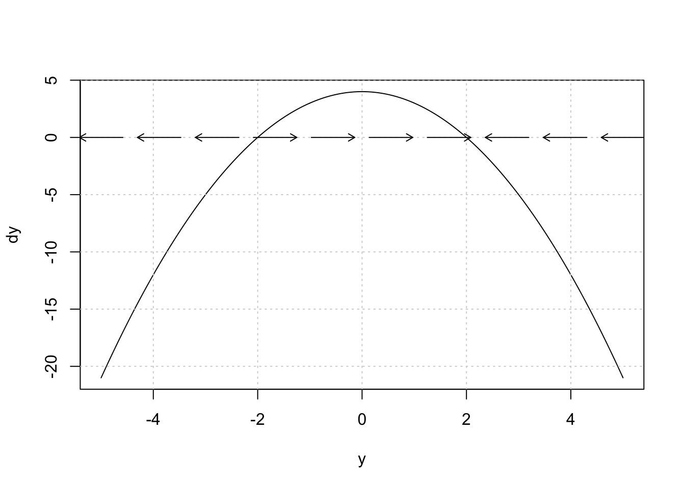
Figure one: Stage Portrait for \(\frac{dy}{dt}=iv-y^two\). The trajectories plotted shows that solutions converge towards \(y=two\), just abroad from \(y=-ii\).
Uniqueness Theorem. The above method assumes \(f\) to exist continuous and differentiable. Hence, these weather guarantee only unique solutions to the autonomous differential equation. Therefore, the solution curves cannot bear upon, expect when they converge at equilibrium points.
Taylor Serial Expansion
The second method for performing stability analyses utilizes the Taylor Serial expansion of \(f\).
Assumptions: Suppose we are a pocket-size distance \(\delta(0)\) abroad from fixed point \(y_*\). And so \(y(0)=y_*+\delta(0)\) and \(y(t)=y_*+\delta(t)\). And so, the Taylor Series of \(f\) can be written every bit the following, such that the \(y^*\) input represents the point where we perform stability analysis:
\[f(y^*+\delta)=f(y^*)+\delta\frac{\partial f}{\fractional y}(y^*)+o(\delta)\]
Example 1. One-Dimesnional ODE
Consider the one-dimensional autonomous ODE: \[\frac{dy}{dt}=y(one-y)(2-y)\]
Flow Field
The following plots the menses field and diverse trajectories, calculation horizontal lines at equilibrium points:
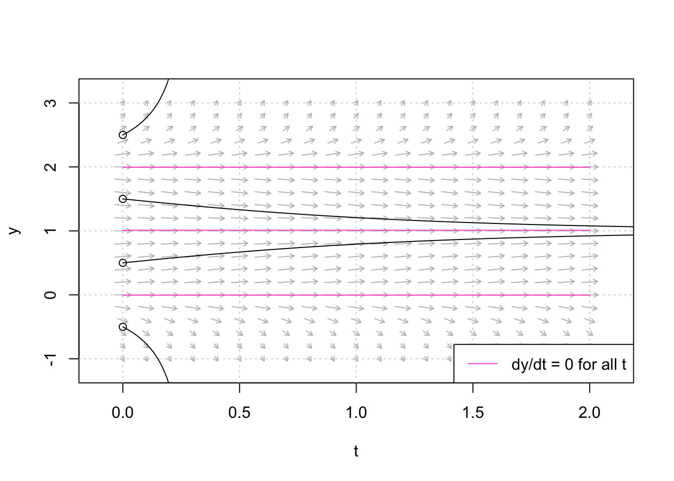
Figure two: The flow field and various trajectories, adding horizontal lines at equilibrium points.
Stock-still Points
The horizontal lines on the graph indicate that three equilibrium points have been identified at \(y^*=0,ane,2\). If nosotros set \(\hat y=0,\) we can analytically solve for the 3 equilibrium points:
\[ \begin{align} y^* (ane-y^* )(two-y^* ) &= 0 \\ y^* &= 0, ane, ii \stop{align} \]
Stability of Fixed Points
Method 1. Stage Portrait
Plotting the phase portrait, nosotros find that \(y^*=0\) and \(y^*=ii\) are unstable; and \(y^*=ane\) is stable
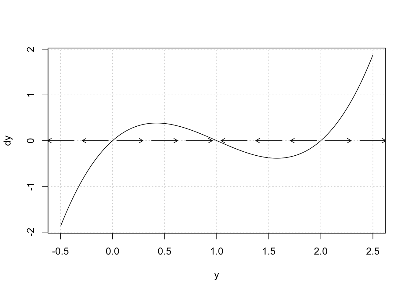
Effigy three: The flow field and various trajectories, adding horizontal lines at equilibrium points.
Method 2. Taylor Series Approach
\[ \brainstorm{align} \frac{dy}{dt}&=y (1-y )(2-y ) \\ &= y^3-4y^two+2y \end{align} \]
Using the Taylor Series arroyo we take:
\[ \begin{marshal} \frac{d}{dy}\left.\left(\frac{dy}{dt}\right)\right|_{y=y^*} &= 3y^{*^2} - 6y^* + 2 = \begin{cases} 2, & \ y^*=0,\\ -one ,& \ y^*=i,\\ two, & \ y^*=2. \cease{cases} \end{align} \]
We draw the same determination as from the phase portrait. We can ostend the Taylor analysis using stability() to check the stability of each equilibrium point:
Hence we reach conclusion as above that \(y^*=ii\) is stable, and \(y^*=-2\) is unstable. Therefore, if \(y(0)>ii\) or \(0<y(0)<2\), then the solution will eventually approach \(y=two\). However, if \(y(0)<0\), \(y\rightarrow-\infty\) as \(t\rightarrow\infty\).
Case 2. Ii-Dimensional ODE
Consider the Lotka-Volterra model, a simple ii species competition model, used in ecology, given by the following:
\[\frac{dx}{dt} = x-xy, \ \frac{dy}{dt} = xy-y\]
a. Plot the velocity field with several trajectories:
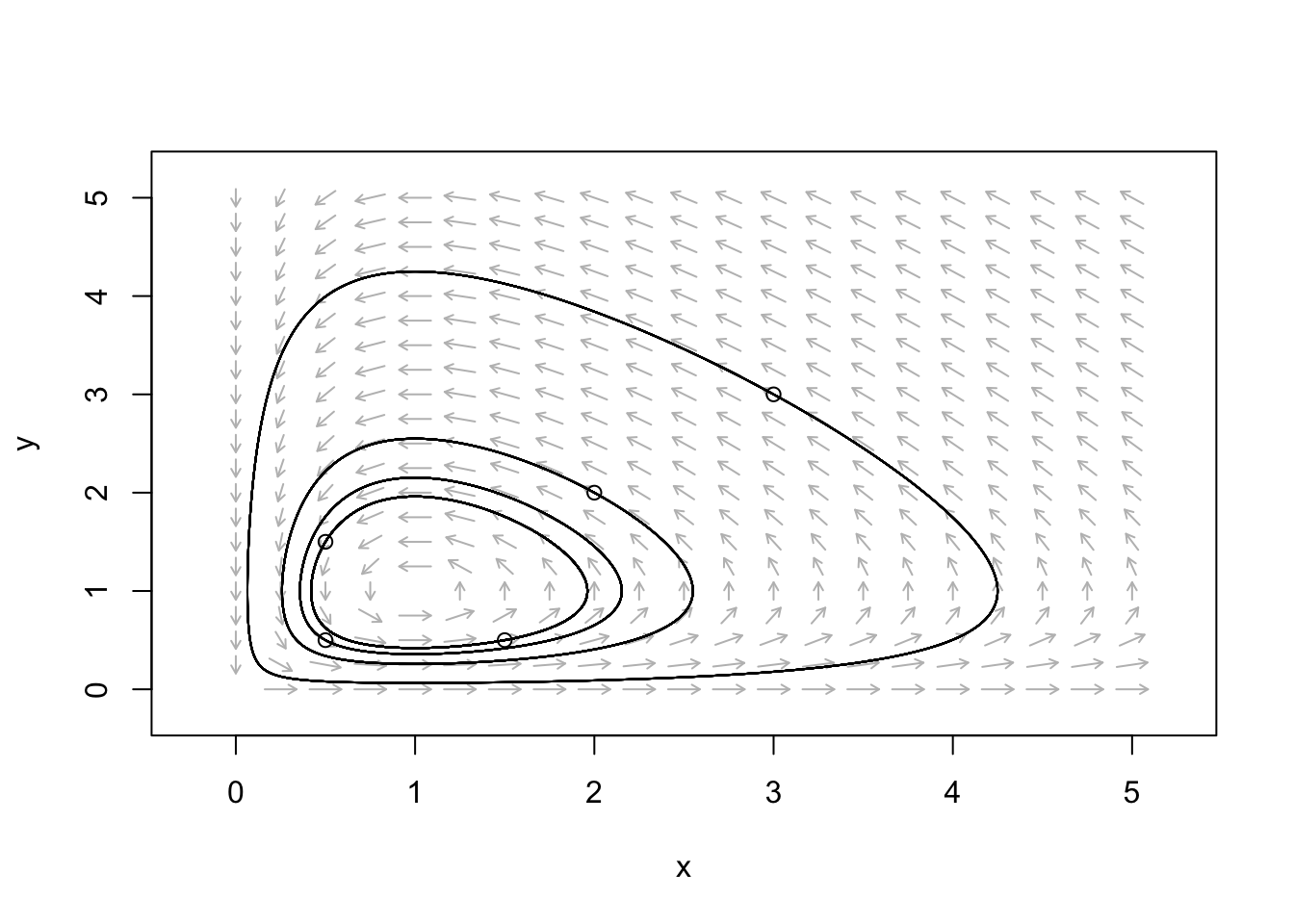
Figure 4: Plot of the velocity field with several trajectories for \(\frac{dx}{dt} = x-xy, \frac{dy}{dt} = xy-y\).
Nullclines
Here, \(x\)-nullclines are divers where \(f(x,y)=0\), while the \(y\)-nullclines are defined where \(g(x,y)=0\). Thus, the \(ten\)- and \(y\)-nullclines define the locations where \(10\) and \(y\) practice not alter with fourth dimension \(t\). When plotting a vector field, it is a adept idea to plot the nullclines start, because the line segments/vectors along the nullclines motility parallel to the \(ten\)- and \(y\)-axes.
b. Summate and Sketch the Nullclines:
\[ \begin{marshal} \mathbf{\dot ten = 0} \\ & \mathrm{x-xy = 0} \ \Longrightarrow \ x(i-y) = 0 \\ & \Rightarrow \mathbf{x=0} \text{ or } \mathbf{y=one},\\ \mathbf{\dot y = 0}\\ & \mathrm{xy-y = 0} \Rightarrow y(ten-one) = 0 \\ & \Rightarrow \mathbf{x=ane} \text{ or } \mathbf{y=0} \end{align} \]
Hence, the fixed points come up out to exist \(\mathrm{(0, 0)}\) and \(\mathrm{(one, ane)}\).
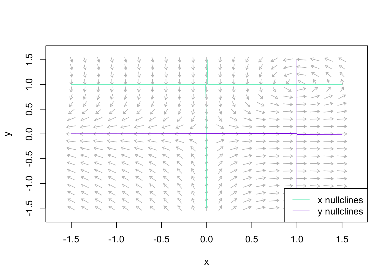
Effigy 5: Sketch of the nullclines for the system of equations \(\frac{dx}{dt} = 10-xy, \frac{dy}{dt} = xy-y\).
Equilibrium points and stability
Equilibrium points defined as the Stock-still points are at \((x_*,y_*)\) where:
\[ f(x^*,y^*)=g(x^*,y^*)=0 \]
c. Taking fractional derivatives we compute the Jacobian at any equilibrium point \((x^∗,y^∗)\):
\[ \brainstorm{marshal} \mathbf{A} &= \brainstorm{bmatrix} \frac{\partial (x-xy)}{\fractional x} & \frac{\fractional (ten-xy)}{\partial y} \\ \frac{\partial (xy-y)}{\partial x} & \frac{\fractional (xy-y)}{\partial y} \end{bmatrix} \\ \\ \mathbf{A}_{(10,y)} &= \begin{pmatrix} \mathrm{1-y} & \mathrm{-x} \\ \mathrm{y} & \mathrm{x-one} \finish{pmatrix} \terminate{align} \]
For the stock-still bespeak \(\mathbf{(0,0)}\)
\[ \mathbf{A}_{(0,0)} = \left.\begin{pmatrix} \mathrm{1} & \mathrm{0} \\ \mathrm{0} & \mathrm{-1} \cease{pmatrix}\right|_{(0,0)} \]
So \(\text{tr}(J)=T=0\) and \(\text{det}(J)=\Delta=-1\); which from our table in a higher place makes \((0,0)\) a saddle betoken.
For the fixed signal \(\mathbf{(ane,1)}\)
\[ \mathbf{A}_{(i,1)} = \left. \begin{pmatrix} \mathrm{0} & \mathrm{-ane} \\ \mathrm{i} & \mathrm{0} \stop{pmatrix}\right|_{(1,1)} \]
Therefore, \(\text{tr}(J)=T=0\) and \(\text{det}(J)=\Delta=i\); which from our table higher up makes \((i,1)\) a middle.
If nosotros expect back at our earlier plot, we can observe trajectories diverging abroad from \((0,0)\), only traversing around \((1,1)\).
d. Plot the Oscillating Nature
Hither we plot \(10\) and \(y\) trajectories against \(t\). For the case of \((x_0,y_0)=(3,4)\) in this example system this results in the following plot which we can view the oscillating nature of \(ten\) and \(y\):
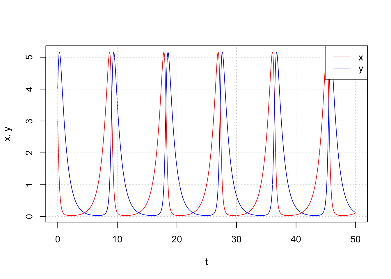
Figure 6: Plot \(x\) and \(y\) trajectories confronting \(t\). In this example, nosotros can view the oscillating nature of \(x\) and \(y\).
Instance iii. Wilson-Cowan Model
The Wilson-Cowan Organisation is a coupled, nonlinear, differential equation for the excitatory and inhibitory populations' firing rates of neurons:
\[\tau_e \frac{dE}{dt} = -E + (k_e - r_e E) \, S_e(c_1 E - c_2 I + P)\]
\[\tau_i \frac{dI}{dt} = -I + (k_i - r_i I) \, S_i(c_3 East - c_4 I + Q),\]
In our numerical search of the steady-state points, we study the cases where the derivatives of \(Due east\) and \(I\) are zero. Since the organization is highly nonlinear, we have to do it numerically. First, nosotros draw the flow field and so describe the nullclines of the arrangement. The \(10\)-nullclines are defined by \(f(x,y)=0\), and the \(y\)-nullclines are divers by \(1000(x, y)=0\). These are the locations where \(ten\) and \(y\) do not change with time.
Limit Cycles. Non-linear systems can exhibit a blazon of behavior known as a limit cycle. If there is only one steady-land solution, and if the steady-state solution is unstable, a limit cycle volition occur. In the following, nosotros define the parameters for satisfying weather condition 18 and twenty equally \(c_1=xvi\), \(c_2 = 12\), \(c_3=15\), \(c_4=three\), \(a_e = 1.three\), \(\theta_e=4\), \(a_i=2\), \(\theta_i = 3.7\), \(r_e=1\) and \(r_i=1\). We tin determine a steady-land solution by the intersection of the nullclines as follows.
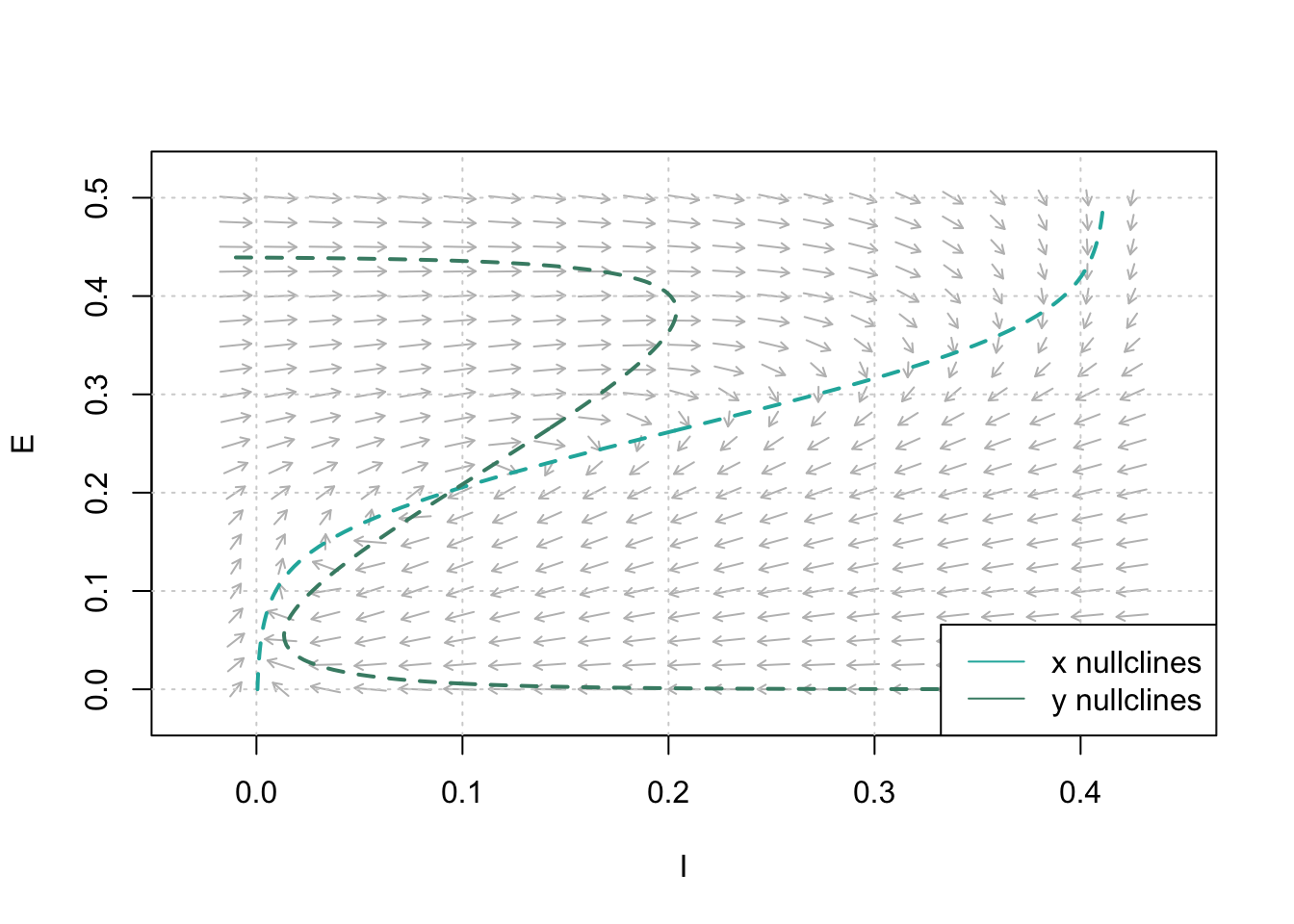
Figure seven: Phase Aeroplane Analysis. Determine the steady-state solution by the nullclines' intersection. Parameters: \(c_1=16\), \(c_2 = 12\), \(c_3=15\), \(c_4=3\), \(a_e = 1.iii\), \(\theta_e=four\), \(a_i=2\), \(\theta_i = iii.vii\), \(r_e=1\), \(r_i=1\).
In the phase airplane, the limit cycle is an isolated airtight orbit, where "closed" means the periodicity of movement, and "isolated" ways the limit of motion, where nearby trajectories converge or deviate. Nosotros can alter our initial values of \(E_0\) and \(I_0\) to obtain different paths in the stage space.
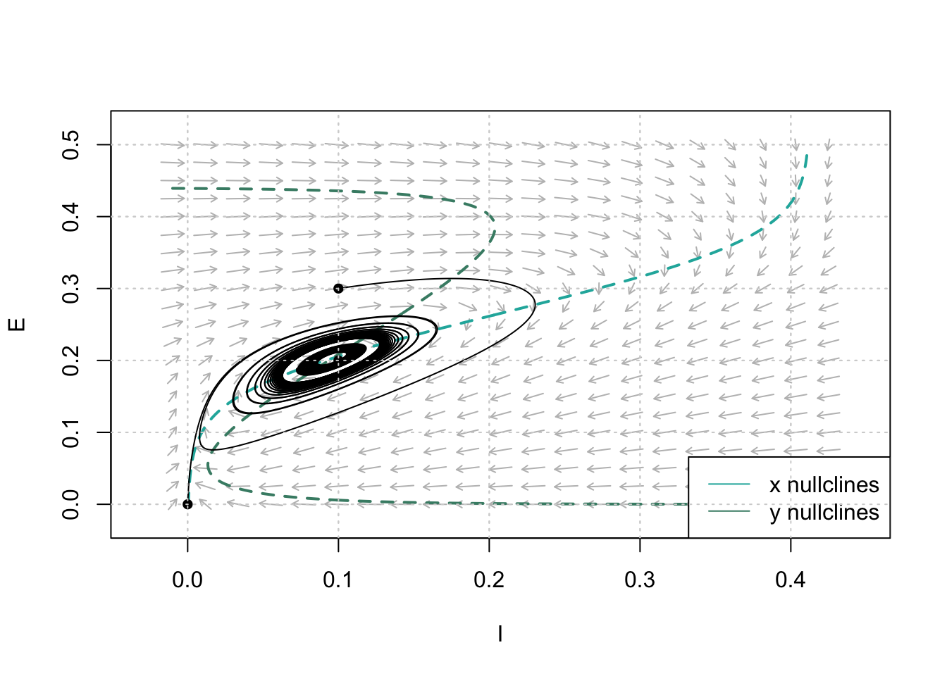
Figure 8: Phase Plane Assay showing limit bike trajectory in response to constant simulation \(P=i.25\). Dashed lines are nullclines. Parameters: \(c_1=xvi\), \(c_2 = 12\), \(c_3=fifteen\), \(c_4=iii\), \(a_e = 1.3\), \(\theta_e=4\), \(a_i=2\), \(\theta_i = 3.7\), \(r_e=1\), \(r_i=1\).
The phase aeroplane analysis illustrates a divisional steady-state solution that is classified as unstable; this is a typical characteristic of a limit cycle. The solution's oscillating behavior, shown in Figure 10, follows typical limit cycle behavior:
- Trajectories almost the equilibrium betoken are pushed farther away from the equilibrium.
- Trajectories far from the equilibrium signal motion closer toward the equilibrium.
We established the resting land \(Due east=0, I=0\) to be stable in the absence of an outside force. Therefore, the neural population only exhibits limit wheel activity in response to a constant external input (P or Q). All in all, the premise of Theorem 3 is that in that location is only ane steady-state, and it must be near the inflection bespeak for a limit bicycle to exist. Therefore, if nosotros study the limit behavior as a function of \(P\), where \(Q=0\), then it follows that:
- At that place is a threshold value of P, and below this threshold, the limit wheel activity cannot occur.
- There is a college value of P, and to a higher place this bound, the arrangement's limit cycle activity volition finish.
- Within the range defined above, both the limit cycle frequency and the average value of \(Eastward(t)\) increases monotonically with respect to \(P\).
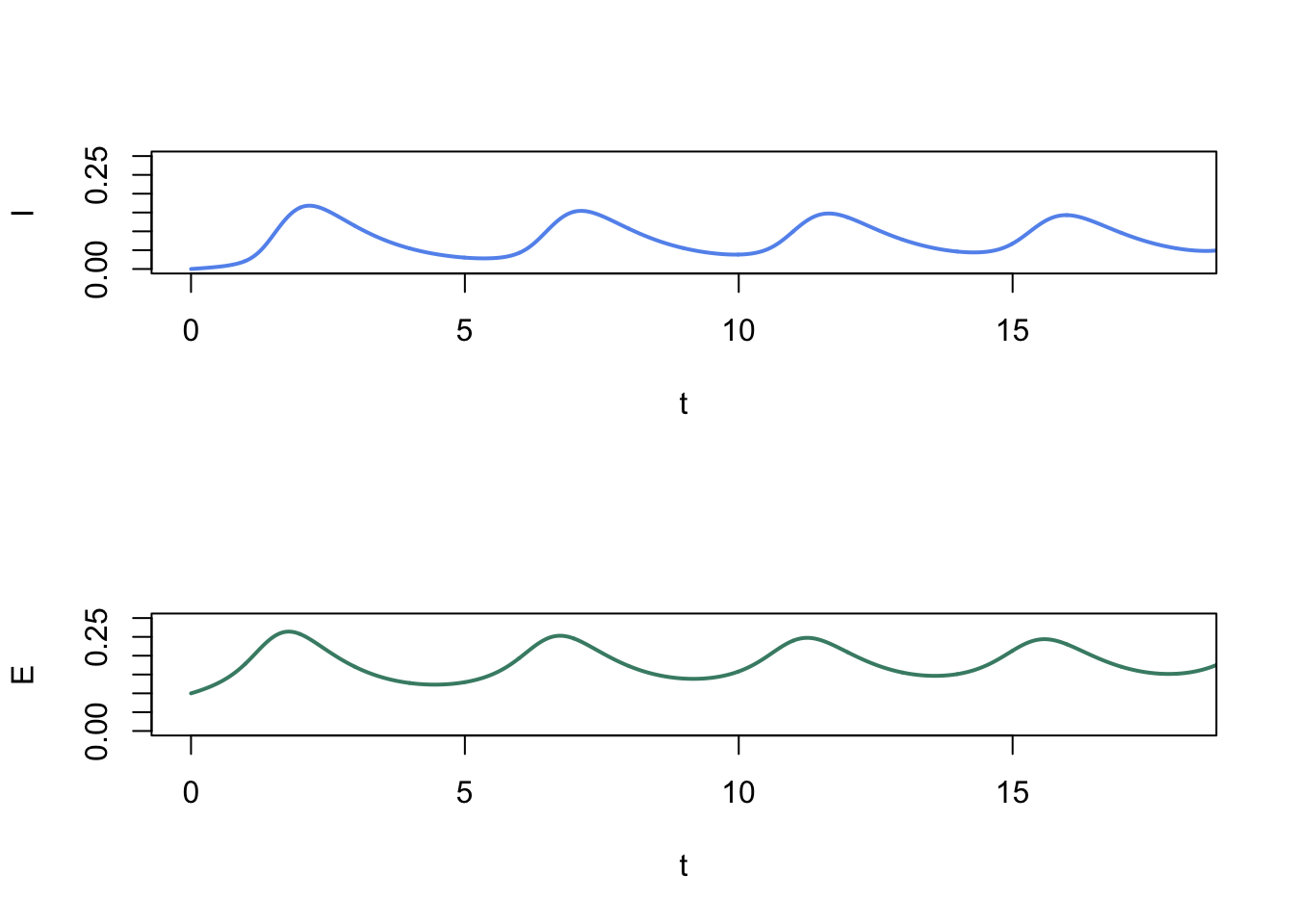
Figure 9: \(I(t)\) and \(Eastward(t)\) for limit wheel shown above. The limit bike depends on the value of \(P\), i.e.\(Q\) existence ready equal to naught.
Summary
The above demonstrates the components necessary to perform qualitative analysis on a i-dimensional autonomous ODE:
- plot the flow field
- plot several trajectories one the flow field
- identify the equilibrium points
- choose a method to determine stability of equilibrium points
Code Appendix
library(knitr) library(phaseR) library(deSolve) library(graphics) library(captioner) library(latex2exp) knitr::opts_chunk$prepare(repeat = FALSE, out.width = 400, fig.align = "center", message = Simulated) fig_nums <- captioner(prefix = "Figure") body_cap <- fig_nums(proper noun = "phase", caption = "Phase Portrait for $\\frac{dy}{dt}=4-y^2$. The trajectories plotted shows that solutions converge towards $y=ii$, but away from $y=-2$.") example1_phasePortrait <- phasePortrait( example1, ylim = c(-5, 5)) body_cap2 <- fig_nums(name = "phase2", caption = "The flow field and various trajectories, adding horizontal lines at equilibrium points.") example2_flowField <- flowField(example2, xlim = c(0, 2), ylim = c(-i, 3), arrangement ="one.dim", add = FALSE) filigree() example2_nullclines <- nullclines(example2, xlim = c(0, 2), ylim = c(-i, iii), organization = "i.dim", col=c("#ff5ccd"), ltw=ii) example2_trajectory <- trajectory(example2, y0 = c(-0.5, 0.v, 1.5, 2.5), tlim = c(0, 4), system = "1.dim") body_cap3 <- fig_nums(proper noun = "phase3", explanation = "The flow field and diverse trajectories, calculation horizontal lines at equilibrium points.") example2_phasePortrait <- phasePortrait( example2, ylim = c(-0.five, ii.v)) example2_stability_1 <- stability( example2, ystar = 0, system = "one.dim") example2_stability_2 <- stability( example2, ystar = ane, system = "one.dim") example2_stability_3 <- stability( example2, ystar = ii, system = "one.dim") body_cap4 <- fig_nums(name = "phase4", explanation = "Plot of the velocity field with several trajectories for $\\frac{dx}{dt} = x-xy, \ \\frac{dy}{dt} = xy-y$.") lotkaVolterra_flowField <- flowField(lotkaVolterra, xlim = c(0, 5), ylim = c(0, 5), parameters = c(1, i, one, one), add together = F) lotkaVolterra_trajectories <- trajectory(lotkaVolterra, y0 = rbind(c(two, ii), c(0.v, 0.5), c(0.5, 1.5), c(1.five, 0.5), c(3, 3)), parameters = c(ane, ane, 1, i), col = rep("black", five), tlim = c(0, 100)) body_cap5 <- fig_nums(name = "phase5", caption = "Sketch of the nullclines for the organization of equations $\\frac{dx}{dt} = x-xy, \ \\frac{dy}{dt} = xy-y$.") lotkaVolterra_flowField <- flowField(lotkaVolterra, xlim = c(-1.v,one.5), ylim = c(-1.v,1.five), parameters = c(1, ane, ane, 1), add together = F) lotkaVolterra_trajectories <- nullclines(lotkaVolterra, xlim = c(-1.v,ane.5), ylim = c(-one.5,i.v), col = c("aquamarine2", "blueviolet"), parameters = c(one, 1, 1, 1), points = 251) body_cap6 <- fig_nums(proper name = "phase6", caption = "Plot $x$ and $y$ trajectories against $t$. In this case, we can view the oscillating nature of $x$ and $y$.") lotkaVolterra_numericalSolution <- numericalSolution(lotkaVolterra, y0 = c(3, four), tlim = c(0, 50), parameters = c(1, one, 1, ane)) se <- function(ten){ ae=1.3 theta_e=four i/(ane+exp(-ae*(ten-theta_e))) } si <- function(ten){ ai=ii theta_i= 3.7 i/(one+exp(-ai*(x-theta_i))) } WilsonCowan2 <- function(t, y, parameters) { # couplings c1 = 16 c2 = 12 c3 = 15 c4 = 3 # Refractory periods rE = i rI = ane # external inputs P = 1.25 Q = 0 ki=0.825 ke=0.88 I <- y[i] Eastward <- y[ii] dy <- c( -I + (ki - rI * I) * si(c3 * E - c4 * I + Q), -East + (ke - rE * Eastward) * se(c1 * E - c2 * I + P)) list(dy) } body_cap8 <- fig_nums(name = "phase8", caption = "Phase Plane Analysis. Determine the steady-state solution by the nullclines' intersection. Parameters: $c_1=16$, $c_2 = 12$, $c_3=15$, $c_4=3$, $a_e = 1.iii$, $\\theta_e=4$, $a_i=two$, $\\theta_i = 3.7$, $r_e=1$, $r_i=1$.") example4_flowField <- flowField(WilsonCowan2, xlim = c(-0.01, .425), ylim = c(0, .5), add = FALSE, ylab = TeX("$E$"), xlab= TeX("$I$"), frac=1) filigree() example4_nullclines <- nullclines(WilsonCowan2, xlim = c(-0.01, .425), ylim = c(0, .five), lty = ii, lwd = 2, col=c("lightseagreen","aquamarine4")) body_cap9 <- fig_nums(proper noun = "phase9", explanation = "Phase Airplane Analysis showing limit bicycle trajectory in response to constant simulation $P=i.25$. Dashed lines are nullclines. Parameters: $c_1=sixteen$, $c_2 = 12$, $c_3=15$, $c_4=iii$, $a_e = i.iii$, $\\theta_e=4$, $a_i=two$, $\\theta_i = 3.7$, $r_e=1$, $r_i=1$.") example4_flowField <- flowField(WilsonCowan2, xlim = c(-0.01, .425), ylim = c(0, .5), add = False, ylab = TeX("$E$"), xlab= TeX("$I$"), frac=1) grid() example4_nullclines <- nullclines(WilsonCowan2, xlim = c(-0.01, .425), ylim = c(0, .5), lty = 2, lwd = 2, col=c("lightseagreen","aquamarine4")) y0 <- matrix(c(0.i,0.3, 0,0, 0.one,0.2), 3, 2, byrow = True) example4_trajectory <- trajectory(WilsonCowan2, y0 = y0, pch=16, tlim = c(0, 100), col="blackness", add=T, ylab=TeX("$E, I$"), xlab=TeX("$t$")) filigree() body_cap10 <- fig_nums(name = "phase10", explanation = "$I(t)$ and $E(t)$ for limit wheel shown above. The limit cycle depends on the value of $P$, i.e. $Q$ being ready equal to goose egg.") example4_solution <- numericalSolution(WilsonCowan2, y0 = c(0.0, 0.1), type = "two", col=c("cornflowerblue", "aquamarine4"), add.legend = T, xlab = TeX("$t$"), ylab = c(TeX("$I$"), TeX("$Due east$")), add.grid = F, tlim = c(0,xx), lwd=2, ylim=c(0,0.3), xlim=c(0,18)) References
[1] Grayling, M. J. (2014). phaseR: An R Bundle for Stage Plane Analysis of Democratic ODE Systems. The R Journal 6 43–51.
sorensonwhoube1981.blogspot.com
Source: https://hluebbering.github.io/phase-planes/